Blog

The AWS Machine Learning (ML) certification is a demanding exam that requires the mastery of AWS IT infrastructure, eg., Kinesis; Statistics, eg., Principal Component Analysis (PCA); an expert level familiarity with AWS SageMaker, a one-stop shop for ML in the AWS console; and modeling with a large variety of algorithms, e.g., XGBoost, K-NN, Linear Learner, etc. In short it requires background in Machine Learning, especially in model tuning, in Statistics, and in the AWS cloud. This post is aimed at those who wishes to both learn the practice of ML in the AWS Cloud, and prepare for the AWS Speciality ML certification.

I suspect that there are many Computer Scientists, IT professionals, Business leaders, and others, who are drawn to the field of ML by the ubiquity of its applications, and by the fact that the cloud opened up the practice of ML to anyone who is interested. I was first introduced to ML by Professor Jan Mycielski, at the University of Colorado at Boulder, who gave me his copy of Perceptrons by Marvin Minsky and Seymour Papert, written in 1969 with a second printing in 1972. The subtitle of Perceptrons is An Introduction to Computational Geometry, and the emphasis of this visionary book (pun intended), which laid the foundations of ML, is on what we would call today object recognition. Indeed, the book’s approach is through the problem of computer vision. Many of the mathematical ideas proposed in the book lay dormant for years, as the hardware needed to run the required computation did not exist at first, and later was the domain of a few scientists with access to mainframes. But today, thanks to the economies of scale of computing allowed by the cloud, anyone can set up a ML training job for a few hundred dollars. Of course, this led to an explosion of the field, and its great applicability in medicine, finance, weather predictions, recommender systems, etc., attracted both enthusiasts and professionals. In my academic and consulting work I have been asked to contribute to problem solving with ML, and the AWS ML Pilot which graciously invited our campus to participate, as well as a recent paper I co-authored on applications of ML to enrollment, spurred me to learn more about ML. A great place to start is the AWS ML certification, as it requires both a theoretical understanding of the field (attractive to academics) and an understanding of the ML pipeline based on AWS tools (attractive to practitioners).

ML Pipeline

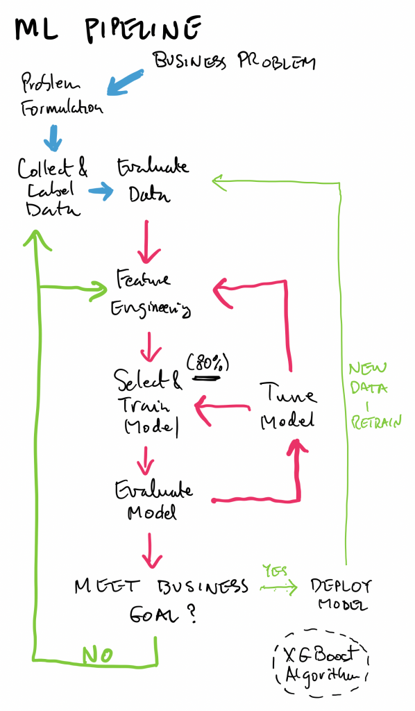
A good way to study for the ML certification is to follow the ML pipeline, which consists of four main stages, which coincide with the four domains of the exam guide (Specialty MLS-C01 Exam Guide v1.2):

1. Data Engineering (20%)
2. Exploratory Data Analysis (24%)
3. Modeling (36%)
4. ML Implementation and Operations (20%)

The percentages indicate the fraction of the exam (65 questions total) dedicated to the given domain. As can be seen, Modeling, consisting of stats, algorithms, tuning and evaluation, is the largest portion. This sets apart the ML certification from other AWS certifications, as it includes a fair amount of theoretical material.

Data Engineering

This domain covers how to create data repositories, eg., a Data Lake, how to ingest data into the repository, and then how to transform the raw data in the repository into data that can be analyzed. This last step is known as a data cleaning operation.

An example of a typical solution is an S3 bucket that hosts the Data Lake, a massive dump collecting data from various sources. This data is then worked on by an Extract-Transform-Load (ETL) application hosted on an Elastic Map Reduce (EMR) cluster. The type of work done here consists in taking the data from a heterogenous set of sources (JSON files, text files, Relational Data Base dumps, images, etc.), and making the data uniform, conforming to a set of conventions described by a table of items (rows) with attributes (columns). The ETL application is typically something like Apache Spark or Apache Hadoop. The data is then written back into the S3 bucket hosting the Data Lake (or possibly a new S3 bucket). The data is now ready, and commonly living in a Pandas table, for consumption by the second stage of the pipeline: Exploratory Data Analysis.

If an exam question has qualifiers such as “set up with little effort” or “minimal management,” this may be an indication that Glue, a serverless data solution, might be preferable to setting up an EMR. This blog post describes how to create a Glue based pipeline.

Here is an interesting blog post on how to preprocess input data before making predictions using a SageMaker Inference Pipelines and Scikit-learn.

Exploratory data analysis

In this stage, data is sanitized. This can mean, for example, taking a variety of date formats (eg., January 23, 2021, 01/23/2021, 23-1-21, etc.) and making them uniform; or, dealing with missing or incomplete data.

ML takes numeric data only, and so all columns have to contain numbers. This may mean taking ordinal data (such as large, medium, small) or nominal data (such as colors), and representing it with numerical data. A subtle point here is that large, medium, small may be translated into 3,2,1, as the numbers represent the order, but the same should not be done with colors where there is no natural ordering to them. In the case of colors, we may want to use one-hot encoding: replace the column with color names with a set of columns with headings for the different colors, as in this example:

Color	Red	Blue	Green
Red	1	0	0
Blue	0	1	0
Green	0	0	1

There are two techniques for dealing with missing data:

1. Remove rows or columns containing missing data
2. Impute missing values, that is, interpolate the missing values by replacing them with the mean of the column, or simply zero, or a little bit more advanced, using regression, very commonly linear regression, which assumes that the data can be estimated well from a linear combination of the existing entries. We will take the opportunity here to mention an excellent source to learn ML: Dive into Deep Learning, and see the 3.1. Linear Regression.

Once the data is sanitized and resides in a table it is possible to perform feature engineering on it. Note here that there are two related terms: attributes and features. Attributes come with the raw data; they are given. Features, on the other hand, are those attributes we select to run the training process. Part of feature engineering is to select appropriate attributes for features.

For example, in detecting fraudulent credit card transactions, it may not be necessary to include the transaction id, which may be generated randomly and carry no information needed to train a model. Thus we drop the transaction id attribute, i.e., it does not become a feature. Another example may be when predicting school enrollments (which students end up coming in the fall based on their applications), it may not be necessary to have both SAT and ACT scores; the two scores may be highly correlated, in which case we only need one of them to train the model. The correlation of two attributes may be found visually with a correlation matrix or a scatter matrix.

The process of removing attributes and/or combining them is called dimensionality reduction, and there are two techniques for it:

1. Principal Component Analysis (PCA)
2. t-Distributed Stochastic Neighbor Embedding (t-SNE)

It may be confusing that PCA and t-SNE are ML algorithms, in fact unsupervised ML algorithms, which are also used to prepare data for ML training. There are difference between PCA and t-SNE, discussed, for example, in this StackExchange post.

Modeling

As with any advanced field in the sciences, it is good to be familiar with the nomenclature, in particular the difference – in the context of ML – between algorithm, model and framework:

1. Algorithm: In general, algorithms are step by step instructions that turn inputs into outputs. Algorithms are a basic object of study of Computer Science, and they have been defined formally (see for example Knuth’s The Art of Computer Programming, Volume 1). In the context of ML, algorithms take as input your data and output a model. For example, in the case of the Linear Regression algorithm, the input is a set of observations, and the output is a linear function with a bias. The SageMaker algorithms, which are the algorithms needed for the exam, can be found here.
2. Model: the interpretation of the data obtained for the sake of predictions, computed with an algorithm. The quality of a model depends on the selection of an appropriate algorithm, the fine tuning process, and the testing.
3. Framework: it is a set of software tools, libraries and interfaces used to compute models with algorithms. For example, the textbook Dive into Deep Learning, proposes three frameworks: MXNET, PYTORCH and TENSORFLOW, all three frameworks are open source, developed by Apache, Facebook and Google, respectively. SageMaker supports all three frameworks, as well as others that can be seen here.

We should also add tensors to the list useful definitions. There seems to be confusion regarding what is a tensor. The confusion may arise from the generality of the concept; many mathematicians have learned the concept in a book such as Spivak’s Analysis on Manifolds; physicists use tensors in mechanics. For the sake of ML, the most useful way to conceptualize tensors is as a generalization of the sequence: scalar (0-dim tensor), vector (1-dim tensor), matrix (2-dim tensor), and now a “cube matrix”, indexed by (i,j,k) is a 3-dim tensor, etc. Indeed they are called ndarray in MXNet. Tensors facilitate the designation of linear transformations in n-dimensional vector spaces. See here for more.

The primary interface to SageMaker is the Jupyter Notebook, a development environment popular with Data Analysts. A Jupyter notebook has a kernel which is the computational engine on which the notebook runs, and both Python and R are natively supported on SageMaker notebooks. When opening a new Jupyter Notebook in SageMaker, the user can select a kernel which supports a given framework.

The first step in the area of Modeling is to cover the different SageMaker algorithms, all listed here. The Table: Mapping use cases to built-in algorithms in the linked document is especially useful, as it lists the algorithms according to use cases. We summarize them here:

1. Supervised Learning:
   • Binary or Multi-class classification; eg., a spam filter
   • Regression; eg., estimating home values
   • Time Series Forecasting; eg., predict sales
     The algorithms here are DeepAR for Time Series, and for the first two, classification and regression, they are: Factorization Machines, K-NN, LL, XGBoost
2. Unsupervised Learning:
   • Feature Engineering (PCA); eg., combine several features into one (component)
   • Anomaly Detection (RCF); eg., find outliers that make model training more difficult, since the “regular” points without outliers lends themselves to a simpler model
   • Embedding high to low dimension (Object2Vec)
   • Clustering or Grouping (K-Means); for discrete groupings within data
   • Topic Modeling (organize docs into topics not known in advanced: LDA, NTM)
3. Textual Classification:
   • Text classification into pre-defined categories (BlazingText)
   • Translation, summary or speach2text (Seq2Seq)
4. Image Processing:
   • Image and multi-label classification
   • Object detection and classification
   • Computer Vision, as in self-driving cars

Hyperparameters are values given to a particular ML algorithm that control its runtime: size of steps, constants, batch sizes, etc. Choosing the right hyperparameters is an art form, and it is acquired by experience, and explained to some extent here. Note that just as we used ML for dimensionality reduction, we can also use ML to tune hyperparameters – this is done with Baysian search and explained in the link just given. In order to help with the understanding of hyperparameters, I recommend reading Linear Regression Implementation from Scratch, where basic hyperparameters such as learning rate, minibatch size, epoch and gradient ascent rate are explained with great examples.

A framework has been selected, and algorithm chosen, a model constructed; how do we know the quality of the model? We need to be able to test against some data that was not used in the training, but for which we know the targets. To that end, it is customary to train the model on 80% of the data, and reserve 10% for validation, used while building the model, and 10% for testing, done at the end. Let’s concentrate on the supervise binary classification case.

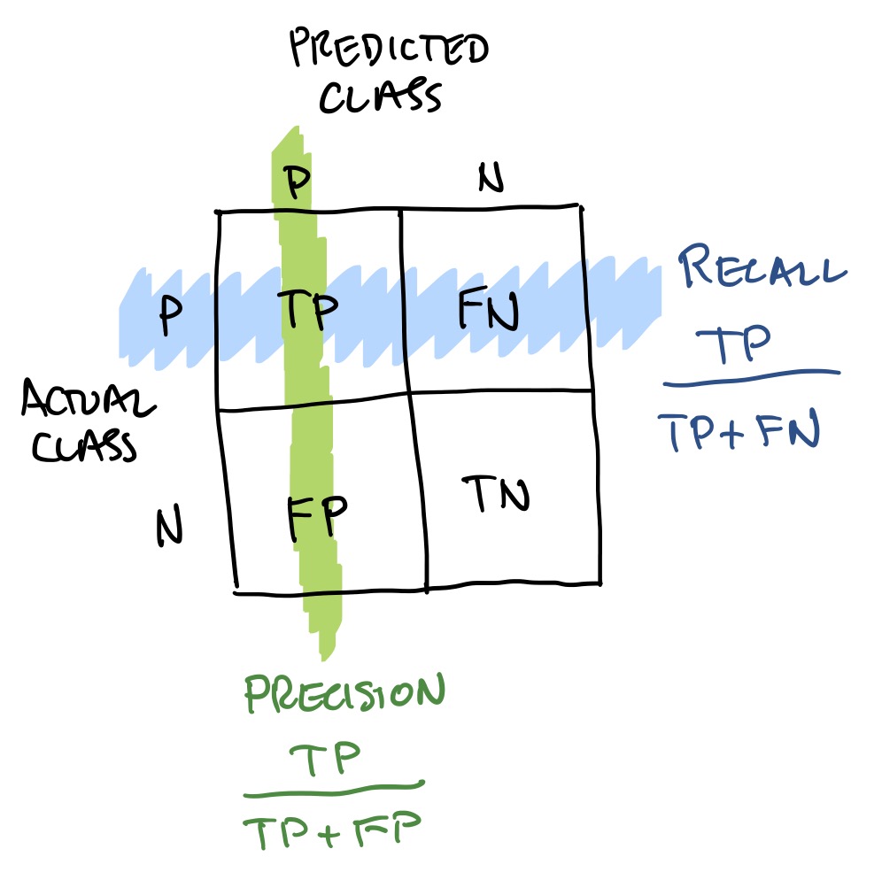
The first step of testing is to build a confusion matrix, which counts how many True Positives (TP), False Negatives (FP), False Positives (FP) and True Negatives (TN) there are. For example, TP are those items which were predicted as positive by the model, and were actually positive; FP are those items which were predicted positive erroneously by the model, since they are in fact negative. There are several metrics associated with a confusion matrix. In the diagram to the left we show Precision, which is TP/(TP+FP), and Recall, which is TP/(TP+FN). Imagine that our model is classifying MRI images according to whether cancer is present or not. It is desirable to identify all images with cancer, even at the cost of having some false positives (the argument being that a dramatic scare is preferable to a tragic neglect of treating a cancer). Thus, in this case high recall can be striven for at the cost of a moderate precision. Note that both recall and precision have a value in [0,1], and a recall close to 1 implies a FN close to zero. There are various other metrics well explained here; Wikipedia has an intro to confusion matrices (note they flipped actual and predicted classes relative to ours).

Implementation and operations

A ML model exists, and now we want to deploy it. In this domain Containers make an appearance, and some familiarity with the concept is necessary (containers are covered in detail in the AWS Developing certification). Another fundamental deployment concept is that of an endpoint. An endpoint is where we attach the model once ready to make inferences; it is a fully managed service that allows real-time inferences via a REST API (see here and here).

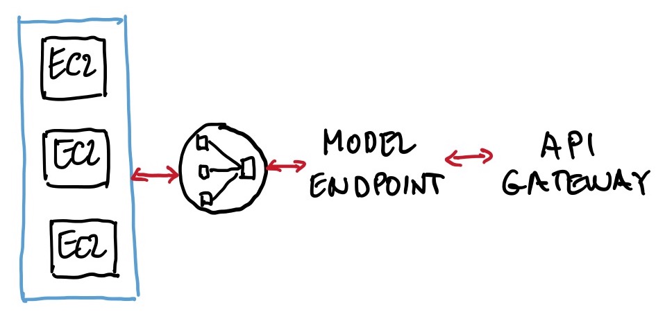
The components of a typical deployment, going right to left in the left figure, is an API managed by AWS API Gateway, that connects to a model endpoint, created with a single line of code in, say, a Python SDK, which then connects to a load balancer which distributes the queries to the model hosted in containers on EC2 instances, possibly spread in several Availability Zones, and part of an auto-scaling group. Note that when a SageMaker model is being trained it is housed in a container, and then the same container, but now with parameters set post-training, is used in the deployment. Also note that endpoints are flexible, in the sense that it takes relatively little effort to have more than one model behind an endpoint (using a shared serving container), with A/B testing supported. The multi-model deployment on a single endpoint, rather then several endpoints, is a good answer to a question that emphasizes low deployment cost, as it reduces deployment overhead since SageMaker manages loading models in memory and scaling them based on the traffic patterns (see here and here).

The above endpoint would work on sporadic queries, but what if the batch or streaming predictions are required? For batch predictions, raw data may be put in an S3 bucket, transformed by an ETL process (EMR + Apache Spark, or Glue), and using a batch transform ingested by the model (see here; note that one of the advantages of batch transform is that you can feed batch data to a model without deploying a persistent endpoint). For streaming predictions, data may be ingested by Kinesis, which connects with SageMaker.; see this blog post. Also see this blog post on Kinesis ingestion of video streams.

Exam Resources

1. AWS official Machine Learning certification site
2. AWS Ramp-Up Guide: Machine Learning
3. AWS Certified Machine Learning – Specialty (MLS-C01) Exam Guide
4. Exam Prep for AWS Certified Machine Learning Specialty
5. GitHub repository with AWS SageMaker examples
6. Great sequence of AWS YouTube videos on SageMaker
7. The Elements of Data Science on AWS Training and Certification is very good
8. Rules of Machine Learning: Best Practices for ML Engineering